Compare sequencing metrics from jafarJ_201021 E coli data
Last updated: 2022-03-25
Checks: 7 0
Knit directory: rare-mutation-detection/
This reproducible R Markdown analysis was created with workflowr (version 1.6.2). The Checks tab describes the reproducibility checks that were applied when the results were created. The Past versions tab lists the development history.
Great! Since the R Markdown file has been committed to the Git repository, you know the exact version of the code that produced these results.
Great job! The global environment was empty. Objects defined in the global environment can affect the analysis in your R Markdown file in unknown ways. For reproduciblity it’s best to always run the code in an empty environment.
The command set.seed(20210916) was run prior to running the code in the R Markdown file. Setting a seed ensures that any results that rely on randomness, e.g. subsampling or permutations, are reproducible.
Great job! Recording the operating system, R version, and package versions is critical for reproducibility.
Nice! There were no cached chunks for this analysis, so you can be confident that you successfully produced the results during this run.
Great job! Using relative paths to the files within your workflowr project makes it easier to run your code on other machines.
Great! You are using Git for version control. Tracking code development and connecting the code version to the results is critical for reproducibility.
The results in this page were generated with repository version 1926d3d. See the Past versions tab to see a history of the changes made to the R Markdown and HTML files.
Note that you need to be careful to ensure that all relevant files for the analysis have been committed to Git prior to generating the results (you can use wflow_publish or wflow_git_commit). workflowr only checks the R Markdown file, but you know if there are other scripts or data files that it depends on. Below is the status of the Git repository when the results were generated:
Ignored files:
    Ignored:    .DS_Store
    Ignored:    .Rhistory
    Ignored:    .Rproj.user/
    Ignored:    analysis/.DS_Store
    Ignored:    scripts/

Untracked files:
    Untracked:  ._.DS_Store
    Untracked:  DOCNAME
    Untracked:  analysis/._.DS_Store
    Untracked:  analysis/cache/
    Untracked:  analysis/calc_nanoseq_metrics.Rmd
    Untracked:  data/
    Untracked:  prototype_code/

Unstaged changes:
    Modified:   analysis/_site.yml
    Modified:   code/efficiency_nanoseq_functions.R
    Modified:   code/load_data.R
Note that any generated files, e.g. HTML, png, CSS, etc., are not included in this status report because it is ok for generated content to have uncommitted changes.
These are the previous versions of the repository in which changes were made to the R Markdown (analysis/ecoli.Rmd) and HTML (docs/ecoli.html) files. If you’ve configured a remote Git repository (see ?wflow_git_remote), click on the hyperlinks in the table below to view the files as they were in that past version.
| File | Version | Author | Date | Message |
|---|---|---|---|---|
| html | 5fd8f9a | Marek Cmero | 2022-03-10 | Build site. |
| Rmd | b257d52 | Marek Cmero | 2022-03-10 | Added MGI vs. Illumina comparison; refactoring ecoli.Rmd code |
| html | cde303e | Marek Cmero | 2022-02-17 | Build site. |
| Rmd | 7cfe3e4 | Marek Cmero | 2022-02-17 | Updated/simplified model |
| html | 36b6bf3 | Marek Cmero | 2022-01-27 | Build site. |
| Rmd | ac440bc | Marek Cmero | 2022-01-27 | Added NanoSeq stats & comparison plots |
| html | bacece1 | Marek Cmero | 2022-01-17 | Build site. |
| Rmd | 47858f3 | Marek Cmero | 2022-01-17 | Added genotype plot |
| html | 02e8ced | mcmero | 2021-12-16 | Build site. |
| Rmd | ce8d35d | mcmero | 2021-12-16 | discordant variant analysis |
| html | f3d146c | mcmero | 2021-12-16 | Build site. |
| Rmd | 7664b09 | mcmero | 2021-12-16 | Updated to handle VCF output |
| html | e5ed9a7 | Marek Cmero | 2021-12-15 | Build site. |
| Rmd | ed42fa9 | Marek Cmero | 2021-12-15 | Added multiQC reports |
| html | de277d9 | Marek Cmero | 2021-12-15 | Build site. |
| Rmd | e610f97 | Marek Cmero | 2021-12-15 | Added ecoli analysis |
Compare sequencing metrics from jafarJ_201021 E coli data
These are extra stats that are not available in the MultiQC reports. These reports can be found below:
library(ggplot2)
library(data.table)
library(dplyr)
library(R.utils)
library(UpSetR)
library(here)
library(vcfR)
library(tibble)
library(stringr)
library(patchwork)
source(here('code/load_data.R'))
source(here('code/plot.R'))qualimap_dir <- here('data/ecoli/jafarJ_201021/QC/qualimap/')
qualimap_cons_dir <- here('data/ecoli/jafarJ_201021/QC/consensus/qualimap/')
variant_dir <- here('data/ecoli/jafarJ_201021/variants')
family_size_stats <- here('data/ecoli/jafarJ_201021_family_sizes.txt')
nanoseq_dir <- here('data/ecoli/jafarJ_201021_nanoseq_results')
samples <- list.files(qualimap_dir)
cov <- load_data(qualimap_dir, 'coverage_across_reference.txt', samples)
ccov <- load_data(qualimap_cons_dir, 'coverage_across_reference.txt', samples)
clip <- load_data(qualimap_dir, 'mapped_reads_clipping_profile', samples)
cclip <- load_data(qualimap_cons_dir, 'mapped_reads_clipping_profile', samples)
vars <- load_data(variant_dir, '.vcf', samples, read.table)
cov_stats <- load_cov_stats(cov, qualimap_dir, samples)
ccov_stats <- load_cov_stats(ccov, qualimap_cons_dir, samples)
fam <- read.delim(family_size_stats, sep='\t')
# TODO: replace these stats with new functions used in compare_MGI_Illumina.Rmd
tsvs <- load_nanoseq_stats(nanoseq_dir)Coverage boxplot
Using coverage summary data from Qualimap (I assume these are summarised to 10kb windows, though I couldn’t find this in the documentation).
# order by median coverage
median_cov <- data.table(cov)[,median(Coverage), by=Sample]
sample_order <- median_cov[order(median_cov$V1)]$Sample
cov$Sample <- factor(cov$Sample, levels = sample_order)
p1 <- ggplot(cov, aes(Coverage, Sample, colour = protocol)) + geom_boxplot() + theme_bw() + ggtitle('Pre-duplex coverage')

median_cov <- data.table(ccov)[,median(Coverage), by=Sample]
ccov$Sample <- factor(ccov$Sample, levels = sample_order)
p2 <- ggplot(ccov, aes(Coverage, Sample, colour = protocol)) + geom_boxplot() + theme_bw() + ggtitle('Duplex coverage')

p1 + p2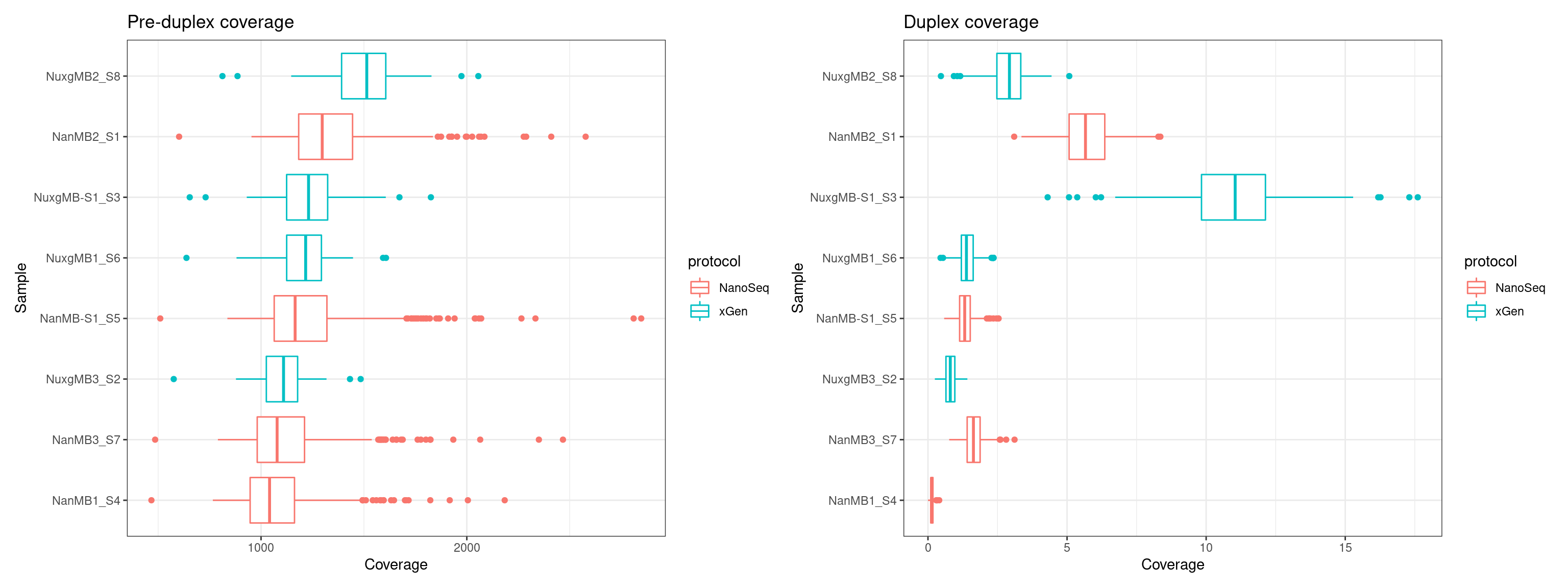
Coverage standard deviation bar plot
ggplot(melt(cov_stats), aes(value, Sample, fill=variable)) +
    geom_bar(stat='identity', position = 'dodge') +
    theme_bw() +
    ggtitle('Coverage std & mean (pre-duplex)')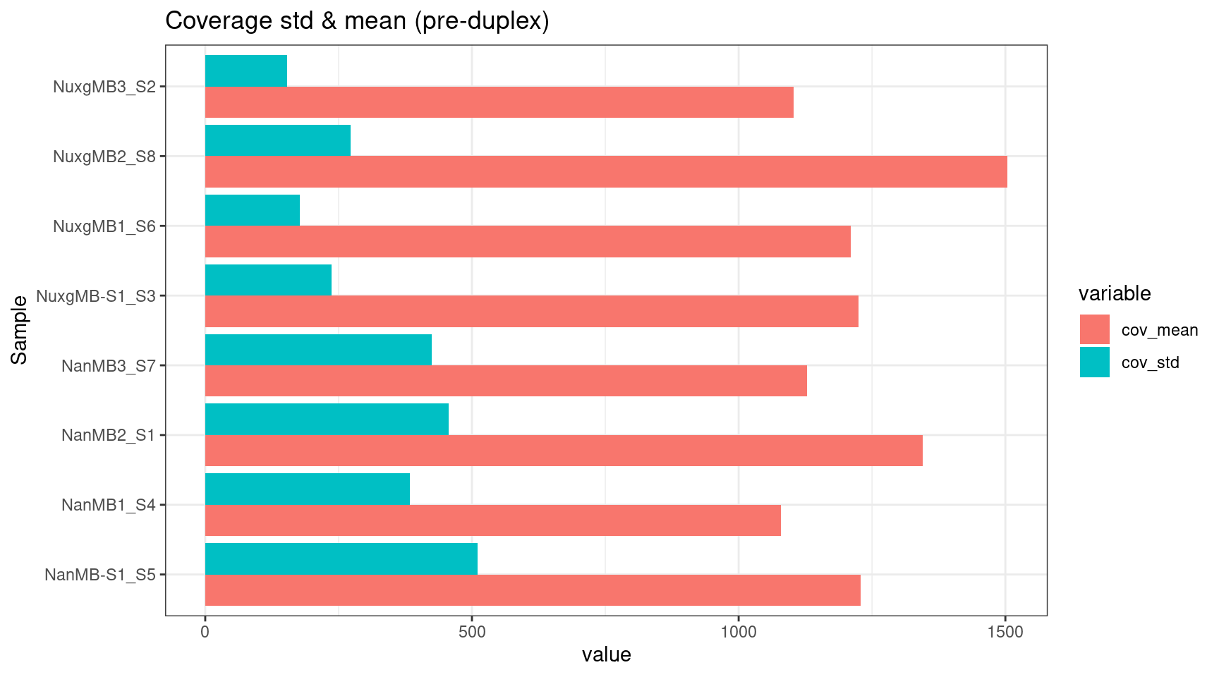
ggplot(melt(ccov_stats), aes(value, Sample, fill=variable)) +
    geom_bar(stat='identity', position = 'dodge') +
    theme_bw() +
    ggtitle('Coverage std & mean (duplex)')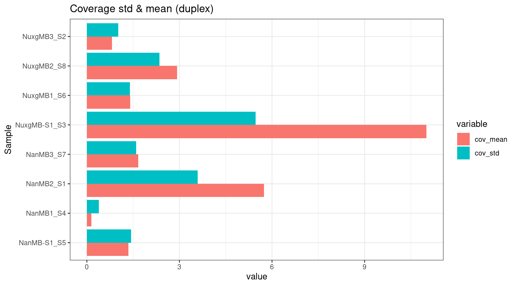
cov_stats$cov_cv <- cov_stats$cov_std / cov_stats$cov_mean
ggplot(cov_stats, aes(cov_cv, Sample)) +
    geom_bar(stat='identity', position = 'dodge') +
    theme_bw() +
    ggtitle('Coverage CV (pre-duplex)')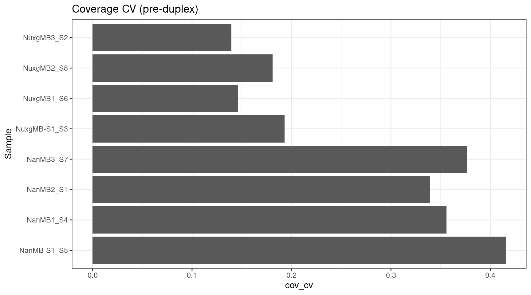
ccov_stats$cov_cv <- ccov_stats$cov_std / ccov_stats$cov_mean
ggplot(ccov_stats, aes(cov_cv, Sample)) +
    geom_bar(stat='identity', position = 'dodge') +
    theme_bw() +
    ggtitle('Coverage CV (duplex)')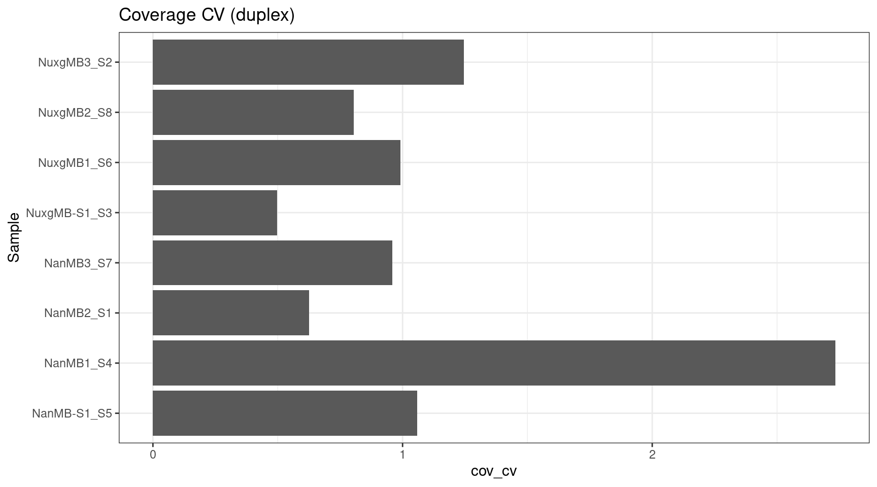
Clipping profile
Pre-duplex reads prior to overlap clipping, but post-UMI removal.
ggplot(clip, aes(X.Read.position..bp., Clipping.profile)) +
    geom_line() +
    theme_bw() +
    xlab('Read position') +
    facet_wrap(~Sample) +
    ggtitle('Pre-duplex clipping profile')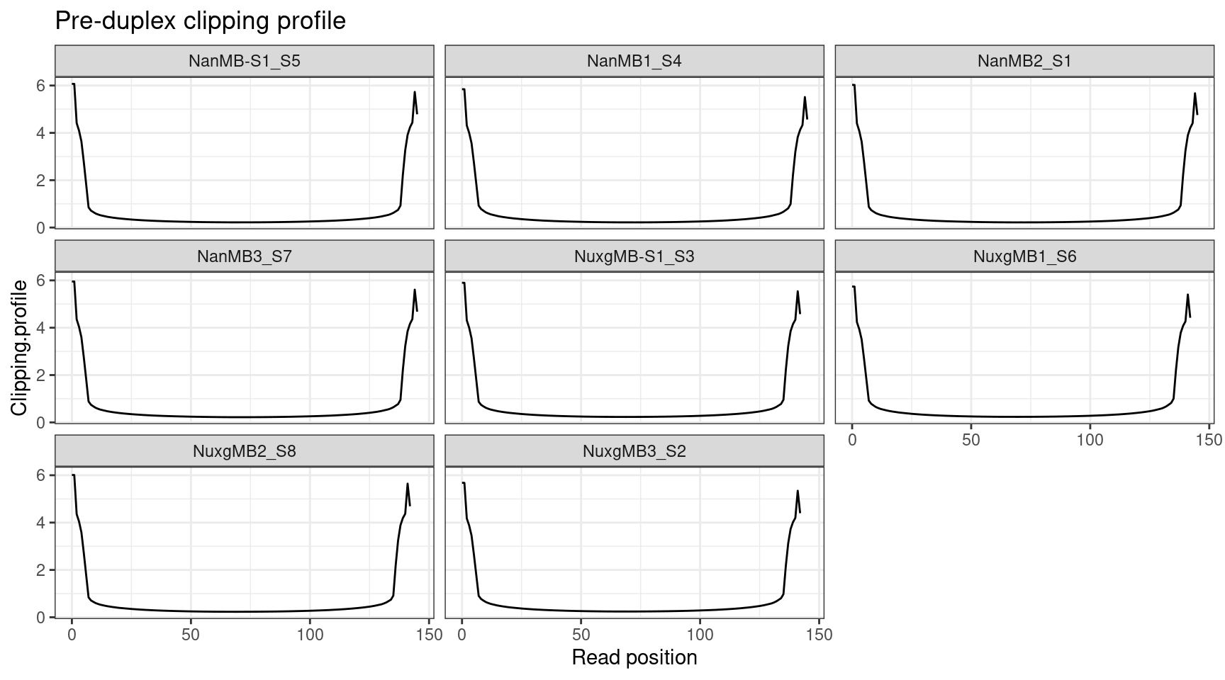
Duplex reads have been clipped to remove read overlap.
ggplot(cclip, aes(X.Read.position..bp., Clipping.profile)) +
    geom_line() +
    theme_bw() +
    xlab('Read position') +
    facet_wrap(~Sample) +
    ggtitle('Duplex clipping profile')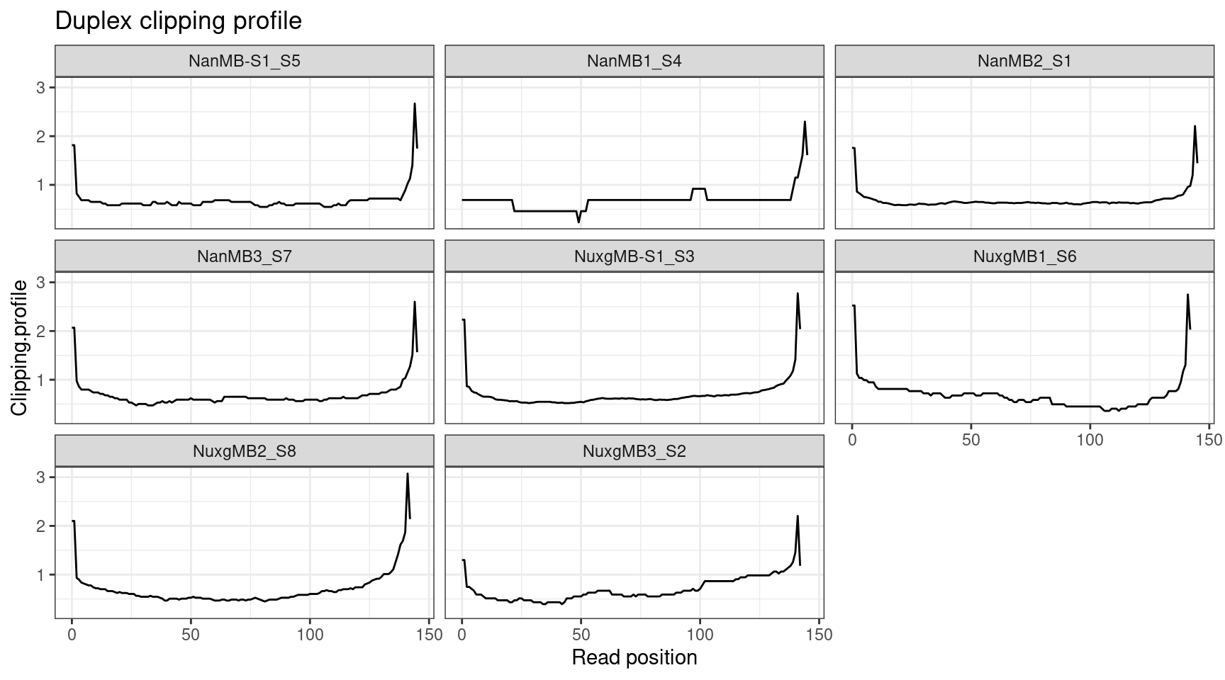
Family size stats (duplex statistics)
- frac_fam_gt1: the fraction of families where family size is greater than one.
- frac_fam_paired: the fraction of paired families (a family on each strand with the same UMI).
- frac_fam_paired_gt1: the fraction of families that are greater than one in size, and also paired.
ggplot(fam, aes(len, sample)) +
    geom_bar(stat='identity') +
    theme_bw() +
    ggtitle('Total family count')
mfam <- reshape2::melt(fam[,c('sample', 'min', 'max', 'mean', 'median')])
ggplot(mfam, aes(value, sample, colour=variable)) +
    geom_point() +
    theme_bw() +
    coord_trans(x='log2') +
    scale_x_continuous(breaks=seq(0, 25, 2)) +
    theme(axis.text.x = element_text(size=6)) +
    ggtitle('Family sizes')
mfam <- reshape2::melt(fam[,colnames(fam) %like% 'frac|sample'])
ggplot(mfam, aes(value, sample, fill=variable)) +
    geom_bar(stat='identity', position='dodge') +
    theme_bw() +
    ggtitle('Family reads + paired statistics')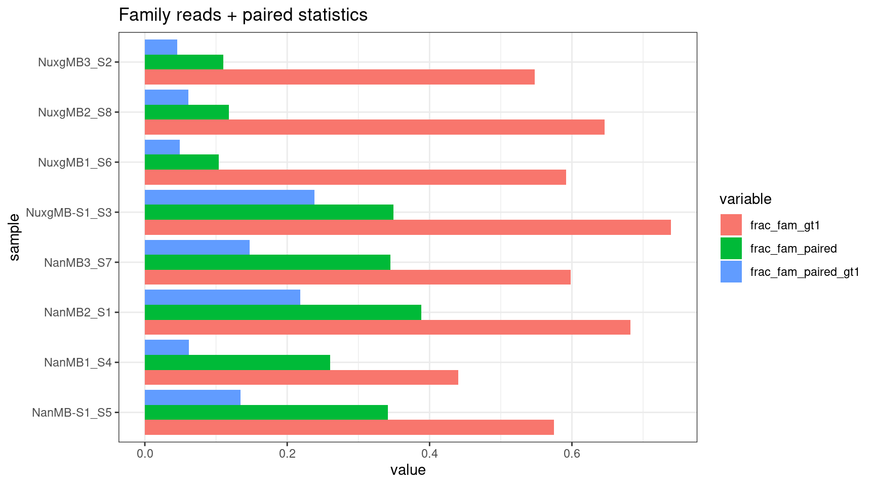
Compare single-read fraction
# extract protocol and nuclease labels
fam$protocol <- 'NanoSeq'
fam$protocol[grep('Nux', fam$sample)] <- 'xGen'
fam$nuclease <- str_split(fam$sample, regex("N(uxg|an)|_")) %>%
                    lapply(., tail, 2) %>% lapply(., dplyr::first) %>% unlist()

mfam <- reshape2::melt(fam[,colnames(fam) %like% 'fam_gt1|sample|protocol|nuc'])
ggplot(mfam, aes(protocol, value)) +
    geom_boxplot() +
    geom_jitter(width=0.1, aes(protocol, value, colour = nuclease)) +
    theme_bw() +
    ggtitle('Fraction families with size > 1 by protocol')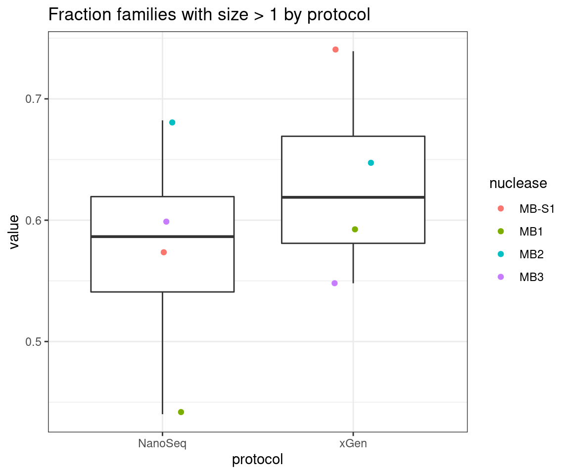
| Version | Author | Date |
|---|---|---|
| 36b6bf3 | Marek Cmero | 2022-01-27 |
ggplot(mfam, aes(nuclease, value)) +
    geom_boxplot() +
    geom_jitter(width=0.1, aes(nuclease, value, colour = protocol)) +
    theme_bw() +
    ggtitle('Fraction families with size > 1 by nuclease')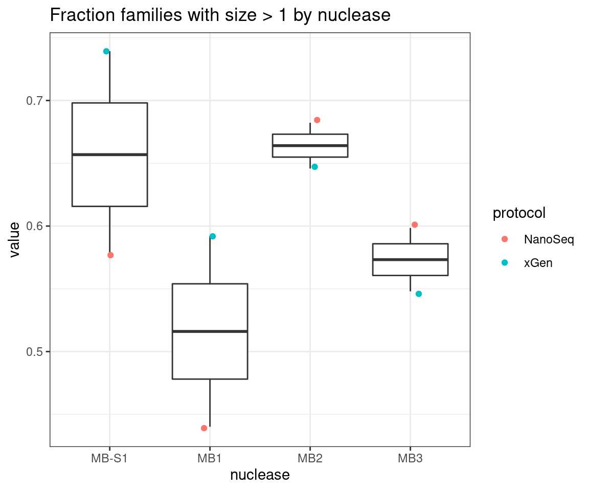
| Version | Author | Date |
|---|---|---|
| 36b6bf3 | Marek Cmero | 2022-01-27 |
Variants
vars$Sample <- strsplit(vars$Sample, '\\.') %>% lapply(., head, 1) %>% unlist()

ulist <- NULL
for(sample in samples) {
    ulist[[sample]] <- vars[vars$Sample %in% sample,]$V2
}

upset(fromList(ulist), order.by='freq', nsets=8)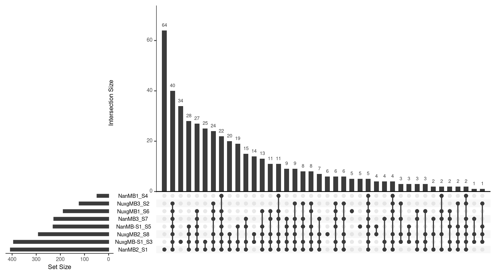
Check how many variants have at least one reference base called.
vcfs <- list.files(variant_dir,
                  full.names = TRUE) %>%
        lapply(., read.vcfR, verbose = FALSE) %>%
        lapply(., vcfR2tidy,
               format_fields = c('GT', 'AD', 'RD'),
               verbose = FALSE)

disc <- lapply(vcfs, function(vcf) {
          has_ref <- vcf$gt$gt_RD > 0
          row <- c(sum(has_ref), nrow(vcf$gt))
          return(row)
        })

disc <- data.frame(disc, row.names = c('has_ref_bases','total_variants')) %>% t() %>%
          data.frame(row.names = 1:nrow(.)) %>%
          add_column(sample=samples)

ggplot(melt(disc), aes(value, sample, fill = variable)) +
  geom_histogram(stat = 'identity', position = 'dodge') +
  theme_bw()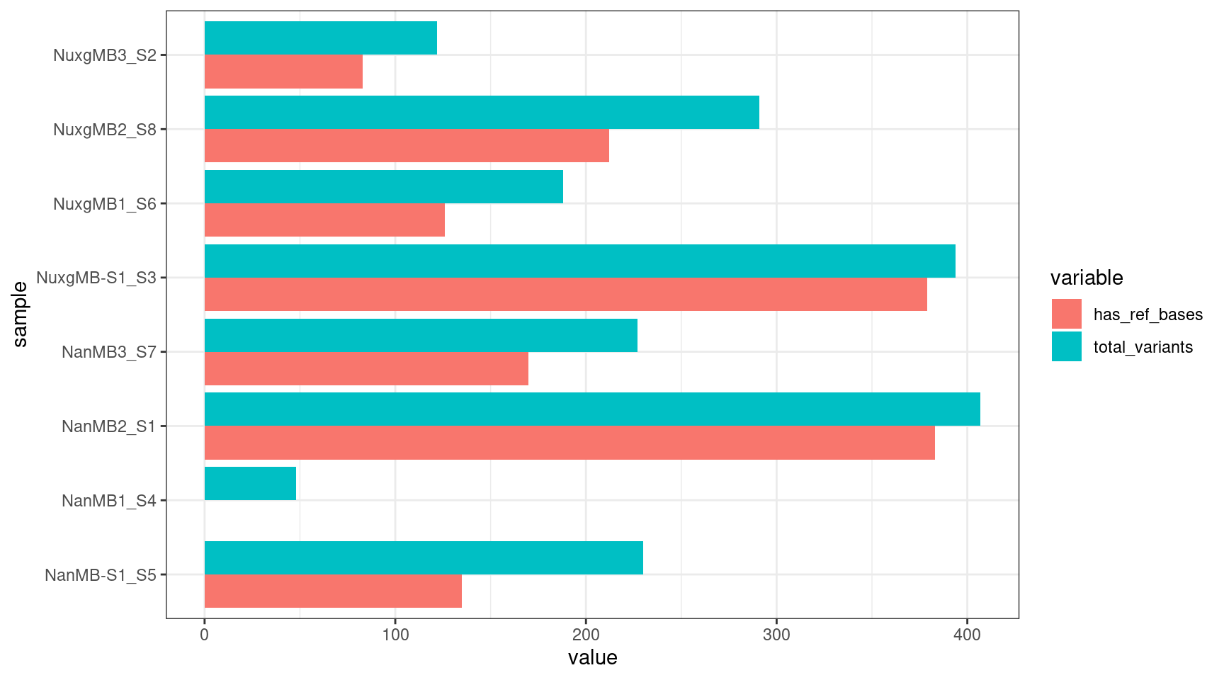
gts <- NULL
for(i in 1:length(samples)) {
    vcfs[[i]]$gt$sample <- samples[i]
    gts <- rbind(gts, vcfs[[i]]$gt)
}

ggplot(gts, aes(sample, fill = gt_GT)) +
    geom_histogram(stat = 'count', position = 'dodge') +
    theme_bw() +
    coord_flip() +
    ggtitle('Variant genotype')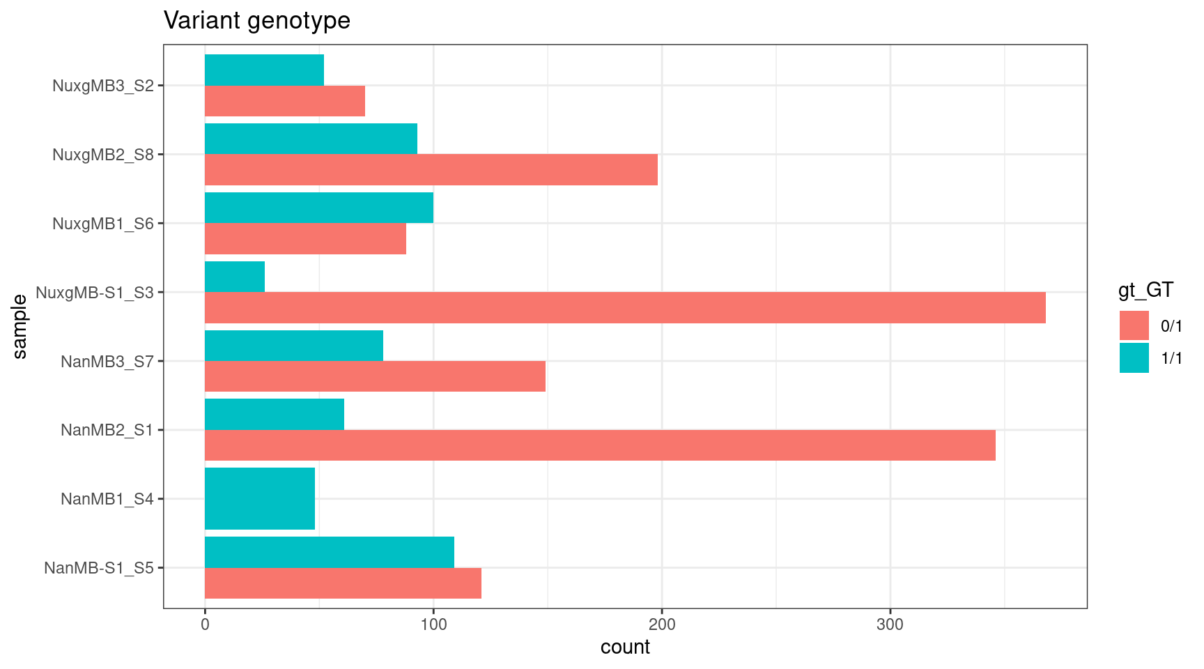
| Version | Author | Date |
|---|---|---|
| bacece1 | Marek Cmero | 2022-01-17 |
Statistics from NanoSeq pipeline
Stats obtained from NanoSeq pipeline.
plot_metric(tsvs, 'READS$', 'Num reads')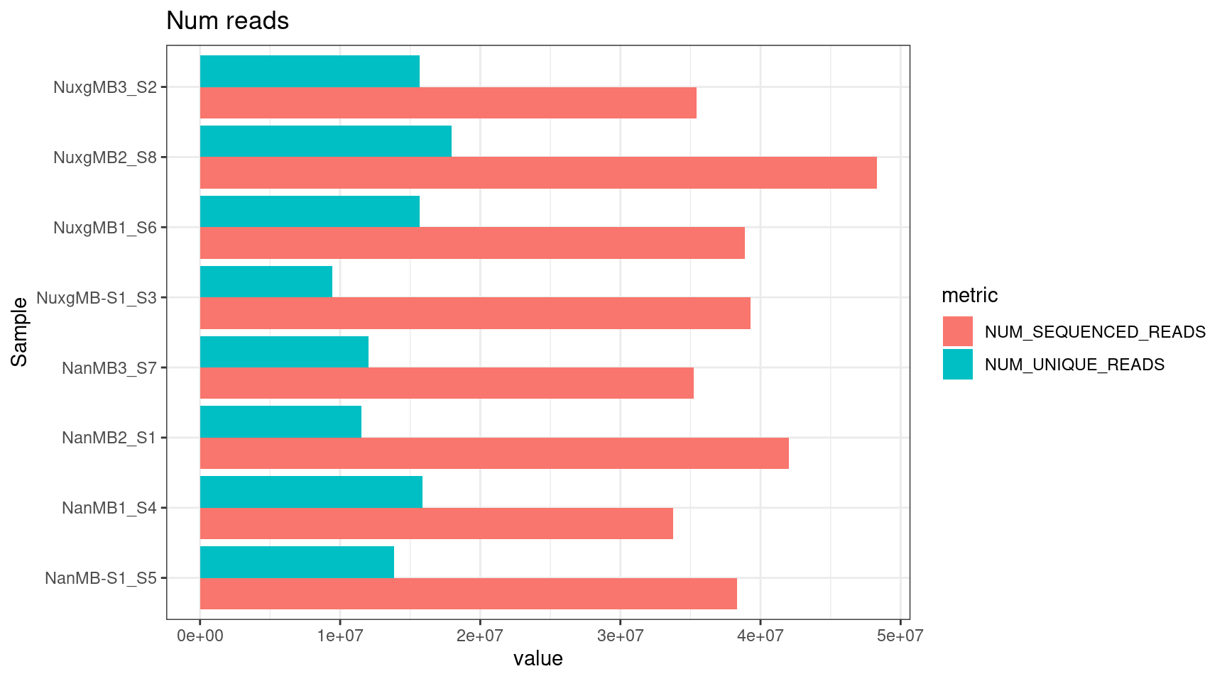
| Version | Author | Date |
|---|---|---|
| 36b6bf3 | Marek Cmero | 2022-01-27 |
plot_metric(tsvs, 'DUPLICATE', 'Duplicate rate (line = optimal)') +
    geom_hline(yintercept = 0.81)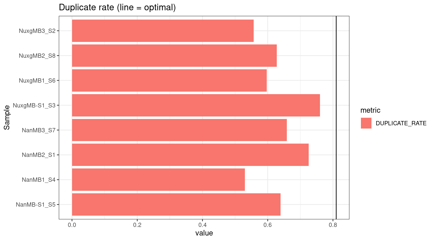
| Version | Author | Date |
|---|---|---|
| 36b6bf3 | Marek Cmero | 2022-01-27 |
plot_metric(tsvs, 'TOTAL', 'Total RBs (read barcodes)')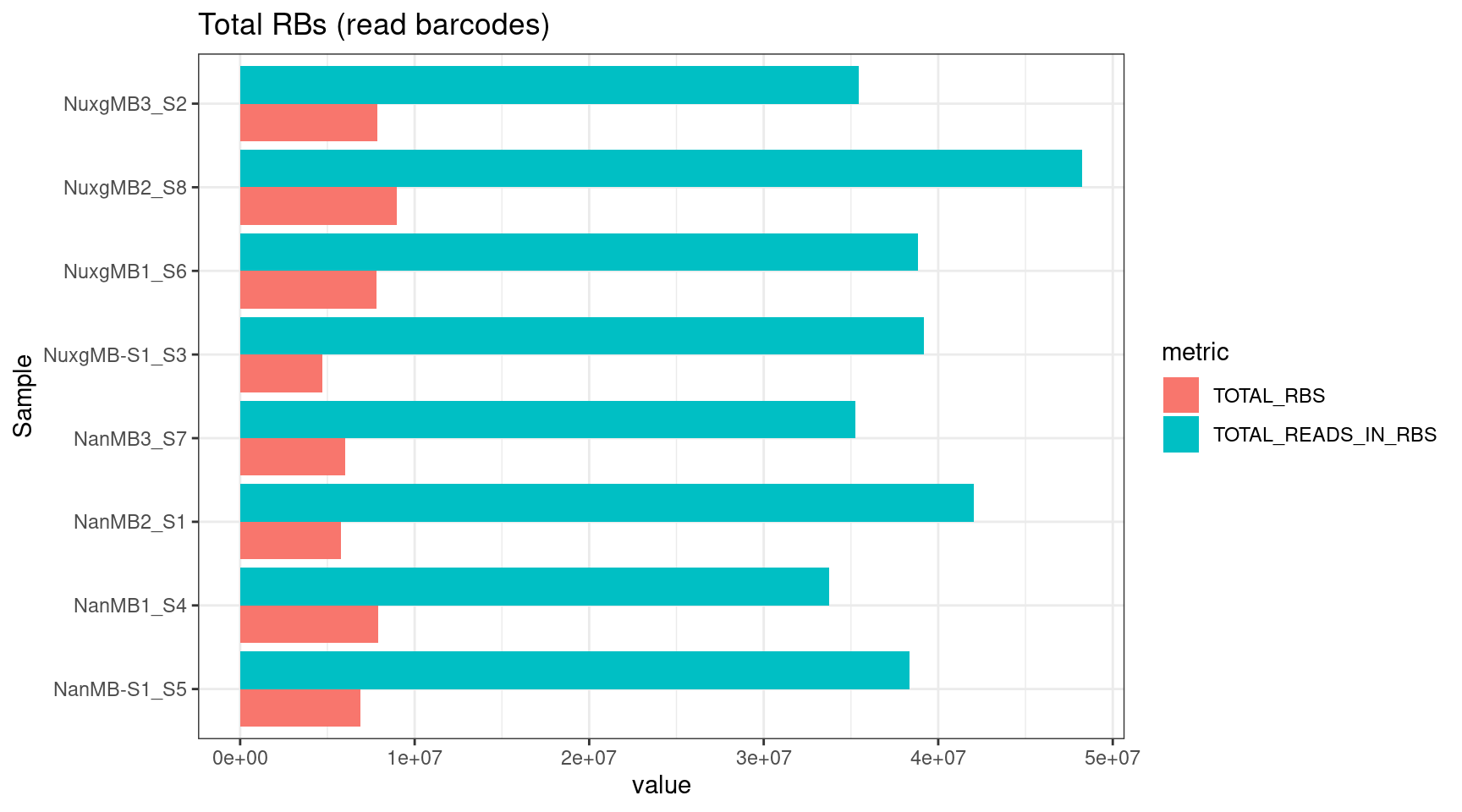
| Version | Author | Date |
|---|---|---|
| 36b6bf3 | Marek Cmero | 2022-01-27 |
plot_metric(tsvs, 'PER', 'Reads per RB')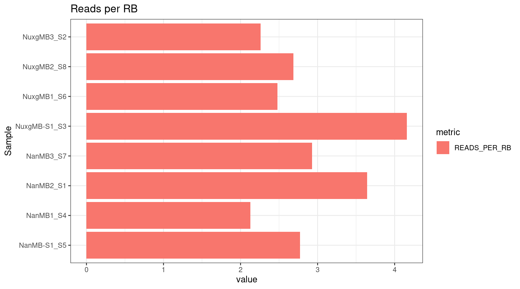
| Version | Author | Date |
|---|---|---|
| 36b6bf3 | Marek Cmero | 2022-01-27 |
plot_metric(tsvs, 'OK', 'OK RBs (2 on each strand)')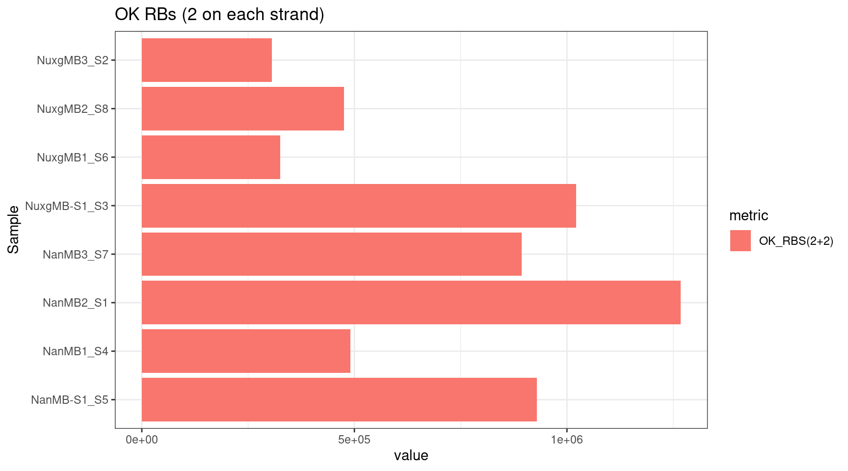
| Version | Author | Date |
|---|---|---|
| 36b6bf3 | Marek Cmero | 2022-01-27 |
plot_metric(tsvs, 'F-EFF',
             'F-EFF (drop out fraction, lines show optimal range)') +
    geom_hline(yintercept = c(0.1, 0.3))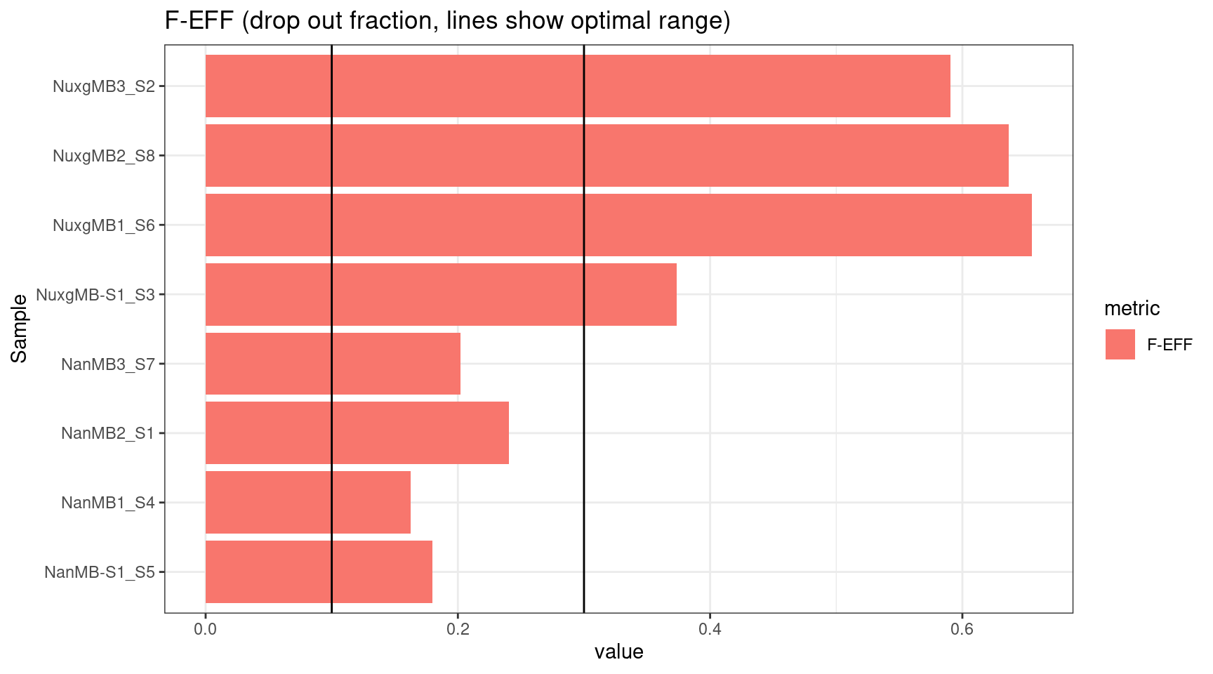
| Version | Author | Date |
|---|---|---|
| 36b6bf3 | Marek Cmero | 2022-01-27 |
plot_metric(tsvs, 'EFFICIENCY','Efficiency (line shows maximised value)') +
    geom_hline(yintercept = 0.07)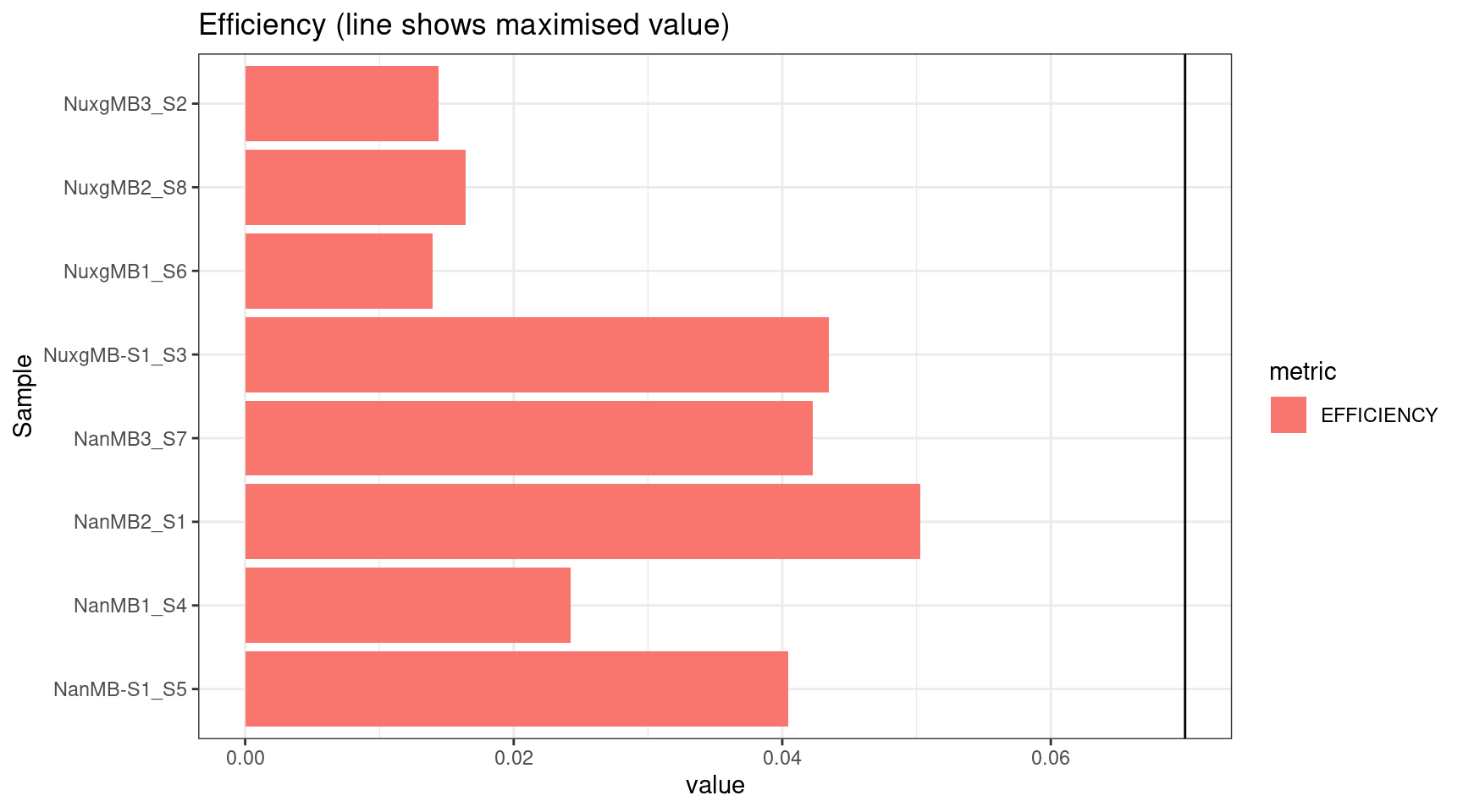
| Version | Author | Date |
|---|---|---|
| 36b6bf3 | Marek Cmero | 2022-01-27 |
plot_metric(tsvs, '(GC_BOTH|GC_SINGLE)', 'GC per strand')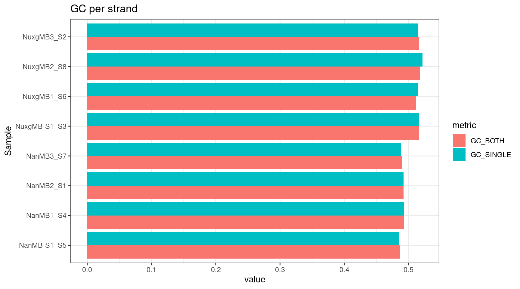
| Version | Author | Date |
|---|---|---|
| 36b6bf3 | Marek Cmero | 2022-01-27 |
Comparison of key stats
# duplicate rate
plot_metric_boxplot(tsvs, 'protocol', 'DUPLICATE', 'Duplicate rate (line = optimal') +
    geom_jitter(width=0.1, aes(protocol, value, colour = nuclease)) +
    geom_hline(yintercept = 0.81)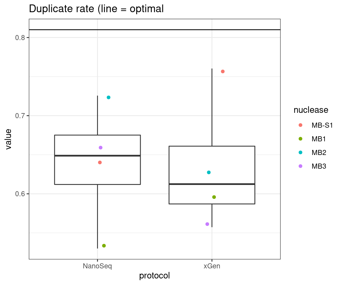
| Version | Author | Date |
|---|---|---|
| 36b6bf3 | Marek Cmero | 2022-01-27 |
plot_metric_boxplot(tsvs, 'nuclease', 'DUPLICATE', 'Duplicate rate (line = optimal') +
    geom_jitter(width=0.1, aes(nuclease, value, colour = protocol)) +
    geom_hline(yintercept = 0.81)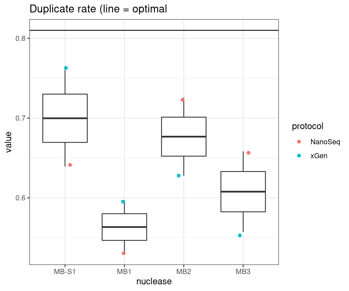
| Version | Author | Date |
|---|---|---|
| 36b6bf3 | Marek Cmero | 2022-01-27 |
# efficiency
plot_metric_boxplot(tsvs, 'protocol', 'EFFICIENCY', 'Efficiency (line = optimal)') +
    geom_jitter(width=0.1, aes(protocol, value, colour = nuclease)) +
geom_hline(yintercept = 0.07) 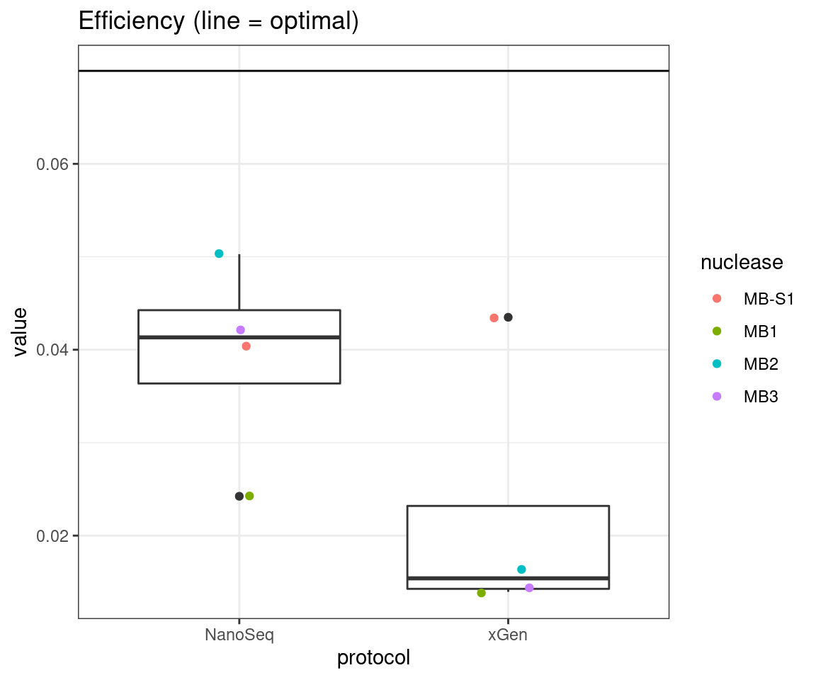
| Version | Author | Date |
|---|---|---|
| 36b6bf3 | Marek Cmero | 2022-01-27 |
plot_metric_boxplot(tsvs, 'nuclease', 'EFFICIENCY', 'Efficiency (line = optimal)') +
    geom_jitter(width=0.1, aes(nuclease, value, colour = protocol)) +
geom_hline(yintercept = 0.07) 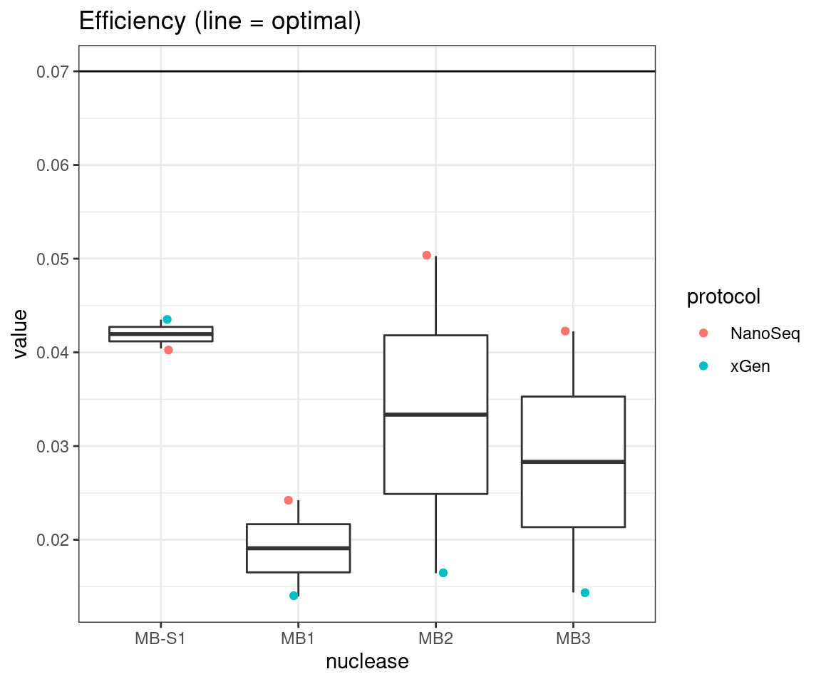
| Version | Author | Date |
|---|---|---|
| 36b6bf3 | Marek Cmero | 2022-01-27 |
# drop out rate
plot_metric_boxplot(tsvs, 'protocol', 'F-EFF', 'Strand drop-out fraction (lines = optimal range)') +
    geom_jitter(width=0.1, aes(protocol, value, colour = nuclease)) +
    geom_hline(yintercept = c(0.1, 0.3))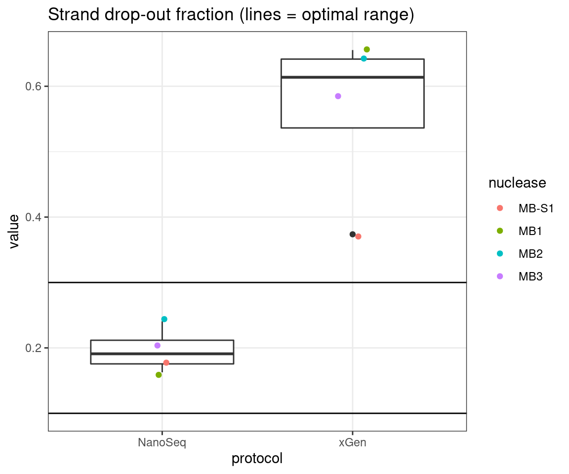
| Version | Author | Date |
|---|---|---|
| 36b6bf3 | Marek Cmero | 2022-01-27 |
plot_metric_boxplot(tsvs, 'nuclease', 'F-EFF', 'Strand drop-out fraction (lines = optimal range)') +
    geom_jitter(width=0.1, aes(nuclease, value, colour = protocol)) +
    geom_hline(yintercept = c(0.1, 0.3))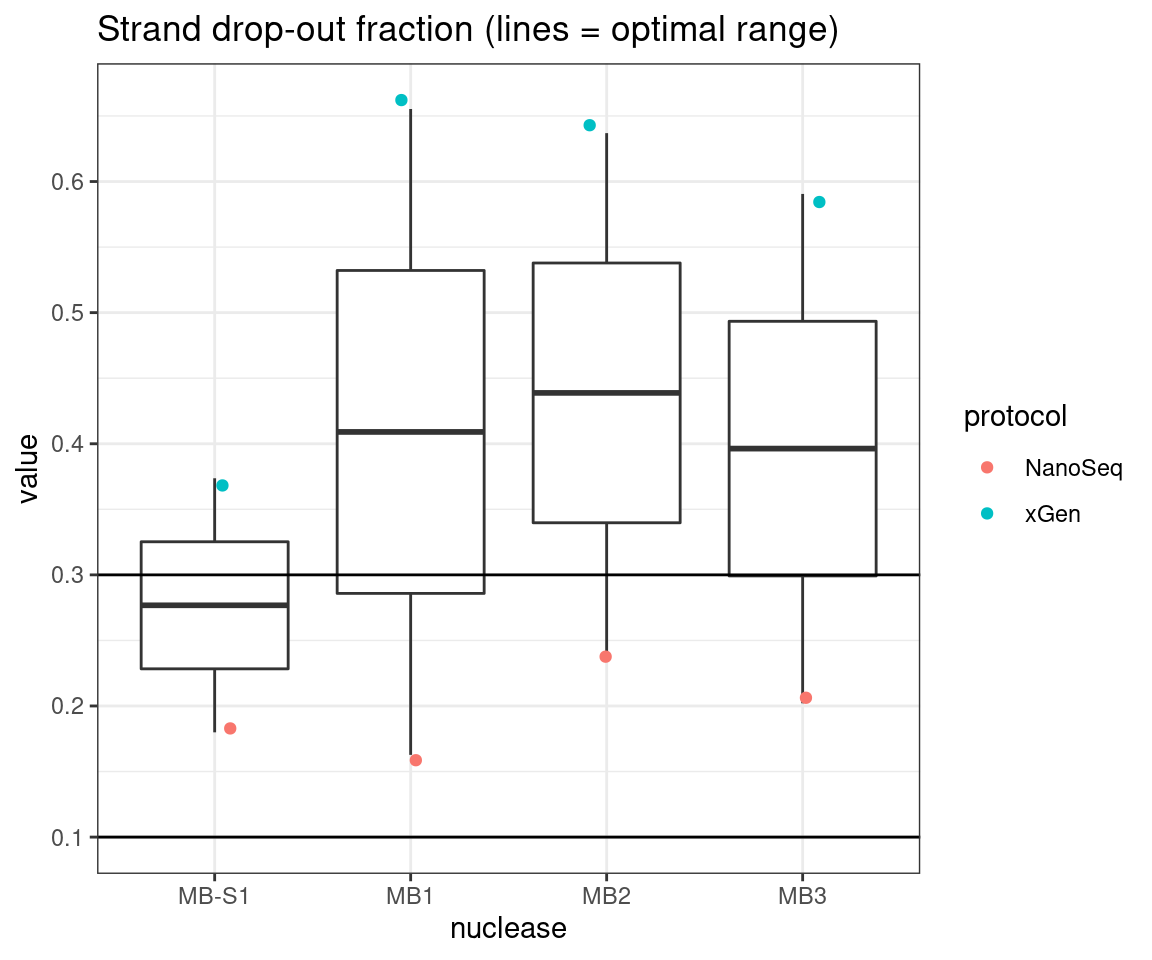
| Version | Author | Date |
|---|---|---|
| 36b6bf3 | Marek Cmero | 2022-01-27 |
# GC deviation between strands
plot_metric_boxplot(tsvs, 'protocol', 'GC_DEV', 'GC deviation (both strands vs. one)') +
    geom_jitter(width=0.1, aes(protocol, value, colour = nuclease))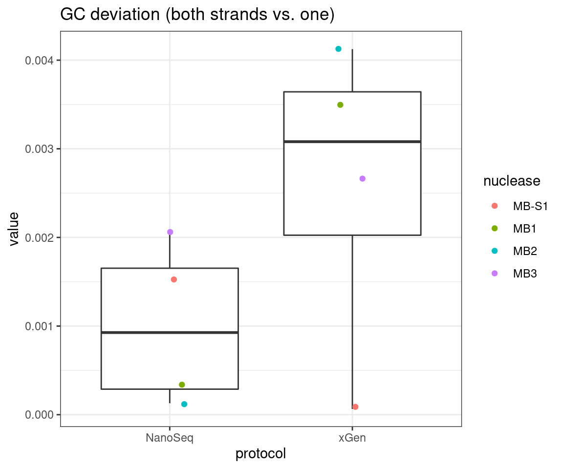
| Version | Author | Date |
|---|---|---|
| 36b6bf3 | Marek Cmero | 2022-01-27 |
plot_metric_boxplot(tsvs, 'nuclease', 'GC_DEV', 'GC deviation (both strands vs. one)') +
    geom_jitter(width=0.1, aes(nuclease, value, colour = protocol))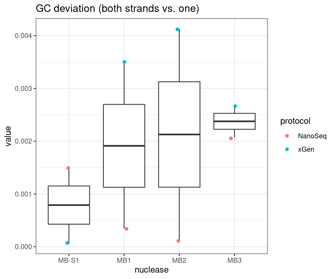
| Version | Author | Date |
|---|---|---|
| 36b6bf3 | Marek Cmero | 2022-01-27 |
sessionInfo()R version 4.0.5 (2021-03-31)
Platform: x86_64-pc-linux-gnu (64-bit)
Running under: CentOS Linux 7 (Core)
Matrix products: default
BLAS: /stornext/System/data/apps/R/R-4.0.5/lib64/R/lib/libRblas.so
LAPACK: /stornext/System/data/apps/R/R-4.0.5/lib64/R/lib/libRlapack.so
locale:
[1] LC_CTYPE=en_US.UTF-8 LC_NUMERIC=C
[3] LC_TIME=en_US.UTF-8 LC_COLLATE=en_US.UTF-8
[5] LC_MONETARY=en_US.UTF-8 LC_MESSAGES=en_US.UTF-8
[7] LC_PAPER=en_US.UTF-8 LC_NAME=C
[9] LC_ADDRESS=C LC_TELEPHONE=C
[11] LC_MEASUREMENT=en_US.UTF-8 LC_IDENTIFICATION=C
attached base packages:
[1] stats graphics grDevices utils datasets methods base
other attached packages:
[1] patchwork_1.1.1 stringr_1.4.0 tibble_3.1.5 vcfR_1.12.0
[5] here_1.0.1 UpSetR_1.4.0 R.utils_2.11.0 R.oo_1.24.0
[9] R.methodsS3_1.8.1 dplyr_1.0.7 data.table_1.14.0 ggplot2_3.3.5
[13] workflowr_1.6.2
loaded via a namespace (and not attached):
[1] Rcpp_1.0.7 ape_5.5 lattice_0.20-44 assertthat_0.2.1
[5] rprojroot_2.0.2 digest_0.6.27 utf8_1.2.2 R6_2.5.1
[9] plyr_1.8.6 evaluate_0.14 highr_0.9 pillar_1.6.4
[13] rlang_0.4.12 whisker_0.4 vegan_2.5-7 jquerylib_0.1.4
[17] Matrix_1.3-2 rmarkdown_2.11 labeling_0.4.2 splines_4.0.5
[21] pinfsc50_1.2.0 munsell_0.5.0 compiler_4.0.5 httpuv_1.6.3
[25] xfun_0.22 pkgconfig_2.0.3 mgcv_1.8-35 htmltools_0.5.2
[29] tidyselect_1.1.1 gridExtra_2.3 memuse_4.2-1 fansi_0.5.0
[33] permute_0.9-5 viridisLite_0.4.0 crayon_1.4.2 withr_2.4.2
[37] later_1.3.0 MASS_7.3-53.1 grid_4.0.5 nlme_3.1-152
[41] jsonlite_1.7.2 gtable_0.3.0 lifecycle_1.0.1 DBI_1.1.1
[45] git2r_0.28.0 magrittr_2.0.1 scales_1.1.1 stringi_1.7.5
[49] reshape2_1.4.4 farver_2.1.0 fs_1.5.0 promises_1.2.0.1
[53] bslib_0.3.0 ellipsis_0.3.2 generics_0.1.1 vctrs_0.3.8
[57] tools_4.0.5 glue_1.4.2 purrr_0.3.4 parallel_4.0.5
[61] fastmap_1.1.0 yaml_2.2.1 colorspace_2.0-0 cluster_2.1.2
[65] knitr_1.33 sass_0.4.0